Galeria Virtual Micornio Arte, obra grafica, documentos antiguos y piezas de coleccion seleccionadas por Roberto Perez Ver catalogo
Galeria Micornio Arte y piezas de coleccion Ver
Galeria Virtual Micornio

Explora arte, obra grafica, documentos antiguos, antiguedades y piezas de coleccion seleccionadas desde el archivo de Roberto Perez.

miércoles, 23 de enero de 2019

backpropagation KERAS


Gran articulo para hacer cuentas con back propagation 


tambien encontre interesante el video de youtube https://www.youtube.com/watch?v=0e0z28wAWfg

Con estos dos puedes sacar el lapiz y papel y hacer cuentas para entender mejor el procedimiento de backpropagation, lo cual hará que te quede mas claros los fundamentos matemáticos

A Step by Step Backpropagation Example

Background

Backpropagation is a common method for training a neural network. There is no shortage of papers online that attempt to explain how backpropagation works, but few that include an example with actual numbers. This post is my attempt to explain how it works with a concrete example that folks can compare their own calculations to in order to ensure they understand backpropagation correctly.
If this kind of thing interests you, you should sign up for my newsletter where I post about AI-related projects that I’m working on.

Backpropagation in Python

You can play around with a Python script that I wrote that implements the backpropagation algorithm in this Github repo.

Backpropagation Visualization

For an interactive visualization showing a neural network as it learns, check out my Neural Network visualization.

Additional Resources

If you find this tutorial useful and want to continue learning about neural networks, machine learning, and deep learning, I highly recommend checking out Adrian Rosebrock’s new book, Deep Learning for Computer Vision with Python. I really enjoyed the book and will have a full review up soon.

Overview

For this tutorial, we’re going to use a neural network with two inputs, two hidden neurons, two output neurons. Additionally, the hidden and output neurons will include a bias.
Here’s the basic structure:
neural_network (7)
In order to have some numbers to work with, here are the initial weights, the biases, and training inputs/outputs:
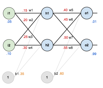
neural_network (9)
The goal of backpropagation is to optimize the weights so that the neural network can learn how to correctly map arbitrary inputs to outputs.
For the rest of this tutorial we’re going to work with a single training set: given inputs 0.05 and 0.10, we want the neural network to output 0.01 and 0.99.

The Forward Pass

To begin, lets see what the neural network currently predicts given the weights and biases above and inputs of 0.05 and 0.10. To do this we’ll feed those inputs forward though the network.
We figure out the total net input to each hidden layer neuron, squash the total net input using an activation function (here we use the logistic function), then repeat the process with the output layer neurons.
Total net input is also referred to as just net input by some sources.
Here’s how we calculate the total net input for h_1:
net_{h1} = w_1 * i_1 + w_2 * i_2 + b_1 * 1
net_{h1} = 0.15 * 0.05 + 0.2 * 0.1 + 0.35 * 1 = 0.3775
We then squash it using the logistic function to get the output of h_1:
out_{h1} = \frac{1}{1+e^{-net_{h1}}} = \frac{1}{1+e^{-0.3775}} = 0.593269992
Carrying out the same process for h_2 we get:
out_{h2} = 0.596884378
We repeat this process for the output layer neurons, using the output from the hidden layer neurons as inputs.
Here’s the output for o_1:
net_{o1} = w_5 * out_{h1} + w_6 * out_{h2} + b_2 * 1
net_{o1} = 0.4 * 0.593269992 + 0.45 * 0.596884378 + 0.6 * 1 = 1.105905967
out_{o1} = \frac{1}{1+e^{-net_{o1}}} = \frac{1}{1+e^{-1.105905967}} = 0.75136507
And carrying out the same process for o_2 we get:
out_{o2} = 0.772928465

Calculating the Total Error

We can now calculate the error for each output neuron using the squared error function and sum them to get the total error:

E_{total} = \sum \frac{1}{2}(target - output)^{2}
Some sources refer to the target as the ideal and the output as the actual.
The \frac{1}{2} is included so that exponent is cancelled when we differentiate later on. The result is eventually multiplied by a learning rate anyway so it doesn’t matter that we introduce a constant here [1].
For example, the target output for o_1 is 0.01 but the neural network output 0.75136507, therefore its error is:
E_{o1} = \frac{1}{2}(target_{o1} - out_{o1})^{2} = \frac{1}{2}(0.01 - 0.75136507)^{2} = 0.274811083
Repeating this process for o_2 (remembering that the target is 0.99) we get:

E_{o2} = 0.023560026
The total error for the neural network is the sum of these errors:
E_{total} = E_{o1} + E_{o2} = 0.274811083 + 0.023560026 = 0.298371109

The Backwards Pass

Our goal with backpropagation is to update each of the weights in the network so that they cause the actual output to be closer the target output, thereby minimizing the error for each output neuron and the network as a whole.

Output Layer

Consider w_5. We want to know how much a change in w_5 affects the total error, aka \frac{\partial E_{total}}{\partial w_{5}}.
\frac{\partial E_{total}}{\partial w_{5}} is read as “the partial derivative of E_{total} with respect to w_{5}“. You can also say “the gradient with respect to w_{5}“.
By applying the chain rule we know that:

\frac{\partial E_{total}}{\partial w_{5}} = \frac{\partial E_{total}}{\partial out_{o1}} * \frac{\partial out_{o1}}{\partial net_{o1}} * \frac{\partial net_{o1}}{\partial w_{5}}
Visually, here’s what we’re doing:
output_1_backprop (4)
We need to figure out each piece in this equation.
First, how much does the total error change with respect to the output?
E_{total} = \frac{1}{2}(target_{o1} - out_{o1})^{2} + \frac{1}{2}(target_{o2} - out_{o2})^{2}
\frac{\partial E_{total}}{\partial out_{o1}} = 2 * \frac{1}{2}(target_{o1} - out_{o1})^{2 - 1} * -1 + 0
\frac{\partial E_{total}}{\partial out_{o1}} = -(target_{o1} - out_{o1}) = -(0.01 - 0.75136507) = 0.74136507
-(target - out) is sometimes expressed as out - target
When we take the partial derivative of the total error with respect to out_{o1}, the quantity \frac{1}{2}(target_{o2} - out_{o2})^{2} becomes zero because out_{o1} does not affect it which means we’re taking the derivative of a constant which is zero.
Next, how much does the output of o_1 change with respect to its total net input?
The partial derivative of the logistic function is the output multiplied by 1 minus the output:

out_{o1} = \frac{1}{1+e^{-net_{o1}}}
\frac{\partial out_{o1}}{\partial net_{o1}} = out_{o1}(1 - out_{o1}) = 0.75136507(1 - 0.75136507) = 0.186815602
Finally, how much does the total net input of o1 change with respect to w_5?
net_{o1} = w_5 * out_{h1} + w_6 * out_{h2} + b_2 * 1
\frac{\partial net_{o1}}{\partial w_{5}} = 1 * out_{h1} * w_5^{(1 - 1)} + 0 + 0 = out_{h1} = 0.593269992
Putting it all together:
\frac{\partial E_{total}}{\partial w_{5}} = \frac{\partial E_{total}}{\partial out_{o1}} * \frac{\partial out_{o1}}{\partial net_{o1}} * \frac{\partial net_{o1}}{\partial w_{5}}
\frac{\partial E_{total}}{\partial w_{5}} = 0.74136507 * 0.186815602 * 0.593269992 = 0.082167041
You’ll often see this calculation combined in the form of the delta rule:

\frac{\partial E_{total}}{\partial w_{5}} = -(target_{o1} - out_{o1}) * out_{o1}(1 - out_{o1}) * out_{h1}
Alternatively, we have \frac{\partial E_{total}}{\partial out_{o1}} and \frac{\partial out_{o1}}{\partial net_{o1}} which can be written as \frac{\partial E_{total}}{\partial net_{o1}}, aka \delta_{o1} (the Greek letter delta) aka the node delta. We can use this to rewrite the calculation above:

\delta_{o1} = \frac{\partial E_{total}}{\partial out_{o1}} * \frac{\partial out_{o1}}{\partial net_{o1}} = \frac{\partial E_{total}}{\partial net_{o1}}
\delta_{o1} = -(target_{o1} - out_{o1}) * out_{o1}(1 - out_{o1})
Therefore:
\frac{\partial E_{total}}{\partial w_{5}} = \delta_{o1} out_{h1}
Some sources extract the negative sign from \delta so it would be written as:
\frac{\partial E_{total}}{\partial w_{5}} = -\delta_{o1} out_{h1}
To decrease the error, we then subtract this value from the current weight (optionally multiplied by some learning rate, eta, which we’ll set to 0.5):

w_5^{+} = w_5 - \eta * \frac{\partial E_{total}}{\partial w_{5}} = 0.4 - 0.5 * 0.082167041 = 0.35891648
Some sources use \alpha (alpha) to represent the learning rate, others use \eta(eta), and others even use \epsilon (epsilon).
We can repeat this process to get the new weights w_6, w_7, and w_8:
w_6^{+} = 0.408666186
w_7^{+} = 0.511301270
w_8^{+} = 0.561370121
We perform the actual updates in the neural network after we have the new weights leading into the hidden layer neurons (ie, we use the original weights, not the updated weights, when we continue the backpropagation algorithm below).

Hidden Layer

Next, we’ll continue the backwards pass by calculating new values for w_1, w_2, w_3, and w_4.
Big picture, here’s what we need to figure out:
\frac{\partial E_{total}}{\partial w_{1}} = \frac{\partial E_{total}}{\partial out_{h1}} * \frac{\partial out_{h1}}{\partial net_{h1}} * \frac{\partial net_{h1}}{\partial w_{1}}
Visually:
nn-calculation
We’re going to use a similar process as we did for the output layer, but slightly different to account for the fact that the output of each hidden layer neuron contributes to the output (and therefore error) of multiple output neurons. We know that out_{h1} affects both out_{o1} and out_{o2} therefore the \frac{\partial E_{total}}{\partial out_{h1}} needs to take into consideration its effect on the both output neurons:
\frac{\partial E_{total}}{\partial out_{h1}} = \frac{\partial E_{o1}}{\partial out_{h1}} + \frac{\partial E_{o2}}{\partial out_{h1}}
Starting with \frac{\partial E_{o1}}{\partial out_{h1}}:
\frac{\partial E_{o1}}{\partial out_{h1}} = \frac{\partial E_{o1}}{\partial net_{o1}} * \frac{\partial net_{o1}}{\partial out_{h1}}
We can calculate \frac{\partial E_{o1}}{\partial net_{o1}} using values we calculated earlier:
\frac{\partial E_{o1}}{\partial net_{o1}} = \frac{\partial E_{o1}}{\partial out_{o1}} * \frac{\partial out_{o1}}{\partial net_{o1}} = 0.74136507 * 0.186815602 = 0.138498562
And \frac{\partial net_{o1}}{\partial out_{h1}} is equal to w_5:
net_{o1} = w_5 * out_{h1} + w_6 * out_{h2} + b_2 * 1
\frac{\partial net_{o1}}{\partial out_{h1}} = w_5 = 0.40
Plugging them in:
\frac{\partial E_{o1}}{\partial out_{h1}} = \frac{\partial E_{o1}}{\partial net_{o1}} * \frac{\partial net_{o1}}{\partial out_{h1}} = 0.138498562 * 0.40 = 0.055399425
Following the same process for \frac{\partial E_{o2}}{\partial out_{h1}}, we get:
\frac{\partial E_{o2}}{\partial out_{h1}} = -0.019049119
Therefore:
\frac{\partial E_{total}}{\partial out_{h1}} = \frac{\partial E_{o1}}{\partial out_{h1}} + \frac{\partial E_{o2}}{\partial out_{h1}} = 0.055399425 + -0.019049119 = 0.036350306
Now that we have \frac{\partial E_{total}}{\partial out_{h1}}, we need to figure out \frac{\partial out_{h1}}{\partial net_{h1}} and then \frac{\partial net_{h1}}{\partial w} for each weight:
out_{h1} = \frac{1}{1+e^{-net_{h1}}}
\frac{\partial out_{h1}}{\partial net_{h1}} = out_{h1}(1 - out_{h1}) = 0.59326999(1 - 0.59326999 ) = 0.241300709
We calculate the partial derivative of the total net input to h_1 with respect to w_1the same as we did for the output neuron:

net_{h1} = w_1 * i_1 + w_3 * i_2 + b_1 * 1
\frac{\partial net_{h1}}{\partial w_1} = i_1 = 0.05
Putting it all together:
\frac{\partial E_{total}}{\partial w_{1}} = \frac{\partial E_{total}}{\partial out_{h1}} * \frac{\partial out_{h1}}{\partial net_{h1}} * \frac{\partial net_{h1}}{\partial w_{1}}
\frac{\partial E_{total}}{\partial w_{1}} = 0.036350306 * 0.241300709 * 0.05 = 0.000438568
You might also see this written as:
\frac{\partial E_{total}}{\partial w_{1}} = (\sum\limits_{o}{\frac{\partial E_{total}}{\partial out_{o}} * \frac{\partial out_{o}}{\partial net_{o}} * \frac{\partial net_{o}}{\partial out_{h1}}}) * \frac{\partial out_{h1}}{\partial net_{h1}} * \frac{\partial net_{h1}}{\partial w_{1}}
\frac{\partial E_{total}}{\partial w_{1}} = (\sum\limits_{o}{\delta_{o} * w_{ho}}) * out_{h1}(1 - out_{h1}) * i_{1}
\frac{\partial E_{total}}{\partial w_{1}} = \delta_{h1}i_{1}
We can now update w_1:
w_1^{+} = w_1 - \eta * \frac{\partial E_{total}}{\partial w_{1}} = 0.15 - 0.5 * 0.000438568 = 0.149780716
Repeating this for w_2, w_3, and w_4
w_2^{+} = 0.19956143
w_3^{+} = 0.24975114
w_4^{+} = 0.29950229
Finally, we’ve updated all of our weights! When we fed forward the 0.05 and 0.1 inputs originally, the error on the network was 0.298371109. After this first round of backpropagation, the total error is now down to 0.291027924. It might not seem like much, but after repeating this process 10,000 times, for example, the error plummets to 0.0000351085. At this point, when we feed forward 0.05 and 0.1, the two outputs neurons generate 0.015912196 (vs 0.01 target) and 0.984065734 (vs 0.99 target).
If you’ve made it this far and found any errors in any of the above or can think of any ways to make it clearer for future readers, don’t hesitate to drop me a note. Thanks!

viernes, 18 de enero de 2019

trading and gambling

Here at Positive Equity we like to consider ourselves gamers.
We chill out during the day with games like Call of Duty, Pro Evolution Soccer, Gran Turismo etc. We have found many similarities between trading and playing video games. Here are some of them.

We need insane Reflex.

Both gamers and traders need to have the reaction time of a house fly dodging a newspaper. The faster the message transfers from brain to mouse click, the better chance you have of getting there before being pwnd.

Our system requirements are the same.

We need high spec computers (sorry, console peasants!), a bucket load of computer memory, The newest solid state hard-drives, powerful graphics cards that we can make melted cheese toasties on and ridiculously big screens to block out the dreaded daylight.
Positive Equity Multiscreens

We need to live a sedentary lifestyle.

Real gamers are often seen as reclusive and anti-social. Gamers would argue that it only applies to the real world.
Real traders by choice give up their social life and a lot of their free time to follow their passion of trading. In either case, Vitamin D is our friend.

It’s a death-match.

One group are over-caffeinated and over-competitive, spending their days battling head to head to win the top of the leader-board. The other group are gamers.

We can suffer from carpal tunnel.

We spend a lot of our time moving a mouse around a pad which can eventually take its toll in the form of wrist, arm and finger pain. It’s also an awkward topic to bring up among friends.

We are affected by latency.

Online gamers need low pings and solid internet connections to successfully compete online and help avoid rage quitting. The lower the ping the quicker the time from mouse click to m-m-m-monsterkill.
Traders need low latency and a solid connection to trade. Lower latency means quicker trade execution. Having a faster line means you are one up on your measly opponents.
Laaag

Gaming gadgets can be trading gadgets.

We both can make use of gaming grade peripherals to have a better competitive edge. From gaming mice that look like ED209 to reality noise cancelling headsets that we think make us look cool and not at all weird.
RAT

We need to take in a lot of information sources at once.

Traders analyse charts and media channels, gamers follow maps and scoreboards. Either way we both take in more information than an average human can handle.

We have to learn to control our temper.

Things can get a bit crazy in the heat of battle. Those who can remain calm and collected will come out the other side unscathed. Those who can’t control their temper are natural losers who resort to childishly shouting about the recent time they spent with their opponent’s mom.

We need to be patient.

Traders are passionate about trading. They live and breathe trading. Not all trading is about crazy markets and constant action. A lot of time is spent in the markets looking for the perfect opportunity to make the click and execute the winning trade. It’s also a great time for stuff like meditation. But more often it’s spent in the gaming room where we can continue owning our opponents.
Video gamers are passionate about gaming. They live and breathe gaming. Not all matches are insane battles without moments of rest. A lot of time may be spent waiting patiently for the perfect moment to make the click and take the head shot. Except if you are a camper. You deserve to die the second you spawn.
This is a top 10 list but there are many more similarities. Why not take your gaming skills to the next level and see if you are fit for a career as a trader?

domingo, 13 de enero de 2019

Robert Kiyosaki

El salario es prestado, hoy esta y mañana no. A mayor nivel de ahorro, mayor nivel de irreverencia.  Juan Diego Gomez

«Este libro trata sobre cómo empecé sin nada y me retiré financieramente libre en menos de diez años. Descubre cómo puedes hacer lo mismo.
Si no quieres pasarte la vida trabajando... este libro es para ti.
¿Por qué no retirarte joven y rico?»
Robert T. Kiyosaki


Robert T. Kiyosaki, autor dePadre rico, padre pobre-el libro sobre finanzas personales nº 1 en el mundo-, revela su experiencia personal para demostrar que sí, que es posible hacerse rico rápidamente y mantener ese nivel económico toda la vida.


En retírate joven y rico, Robert T. Kiyosaki nos revela una vez más los secretos que aprendió junto a su padre rico y los pone a nuestra disposición para que alcancemos la libertad financiera. Además, relata su propia historia de inversionista, gracias a la cual pudo retirarse con absoluta independencia en menos de 10 años. Este libro se dirige a todas aquellas personas cuyo plan no consiste en permanecer toda la vida dentro del mundo laboral, sino que buscan conquistar la autonomía financiera de forma rápida y para siempre. El autor de padre rico, padre pobre, enseña a las personas a hacerse millonarias... Por eso lo llaman el maestro millonario. -la razón principal por la cual las personas luchan por salir adelante es porque, aunque han pasado años en los colegios, no aprendieron nada acerca del dinero. El resultado es que aprenden a trabajar por el dinero... Pero nunca a tener dinero trabajando para ellos-.


https://www.rankia.mx/blog/mejores-afores/2810415-mejores-afores-para-2019


Mejores Afores para 2019


En el siguiente espacio se determinarán cuáles serán las mejores afores para 2019, para ello, se analizarán las afores en cada una de las siefores a fecha de diciembre de 2018. Indicaremos cuáles han sido las afores más y menos rentables el pasado año, atendiendo al rendimiento neto que han obtenido. También tendremos en cuenta el rendimiento neto que han obtenido en relación a las comisiones y los servicios que prestan. Las mejores afores para 2019 son Afore Profuturo, PensionISSSTE, Inbursa y Citibanamex.


http://shop.oreilly.com/product/9780596006778.do

Online Investing Hacks

100 Industrial-Strength Tips & Tools


Publisher: O'Reilly Media
Release Date: March 2010
Pages: 512


For the geek who's an investor, and the investor who's a geek, we present Online Investing Hacks, 100 industrial-strength, bleeding edge tips, tools and techniques for analyzing and managing online portfolios. Individual investors have become more computer-literate and technology-dependent than ever before. Whether you're looking for suitable investments, studying alternatives, or managing your portfolios, you need data. The Internet can be a goldmine of financial data and research, but today's online investors also use spreadsheets, databases, and financial applications to select, study and manage investments. If your proficiency has grown to the point where you crave industrial-strength tips and tools to turbo-charge your efforts, this is the book for you. Online Investing Hacks covers:
  • Screening Investments
  • Collecting Data
  • Fundamental Analysis
  • Technical Analysis
  • Executing Trades
  • Investing in Mutual Funds
  • Portfolio Management
  • Updating Stock Data
  • Financial Planning
Other books for managing online investing are either out of date, are for beginners and don't go beyond the most basic advice, or are so dull and boring they squeeze that last bit of fun out of the topic. Online Investing Hacks is for the customer who wants to know the latest techniques, to go beyond the basics, who gets jazzed by cool online tools and services, and who actually wants to have a bit of fun while trying to strike it rich (or at least not lose their shirt).

Galeria Virtual Micornio

Galeria Virtual Micornio

Arte, obra grafica, documentos antiguos y piezas de coleccion seleccionadas desde Mexico.



























